3. From numbers to figures

Some analyses give one value per atom, as in the last lesson. Others describe the whole system. Their results are plain NumPy arrays, ready for a figure. This lesson shows how heat looks in the radial distribution function of copper.

A crystal and a shaken crystal

Atoms at a finite temperature move about their sites. Random displacements give a rough picture of that. Remember that with_columns also replaces columns, the positions too:

import numpy as np
from mdapy.build import build_crystal

crystal = build_crystal("fcc", 3.615, elements="Cu", repeat=(12, 12, 12))
rng = np.random.default_rng(1)
shaken = crystal.with_columns(
    positions=crystal["positions"] + rng.normal(0, 0.15, (len(crystal), 3))
)

A result of the whole system

The pattern is the one you know: parameters, then compute. There is no column to add, as there is one curve for all the atoms:

from mdapy.analysis import RadialDistributionFunction

analysis = RadialDistributionFunction(r_max=8.0, bins=200)
cold = analysis.compute(crystal)
hot = analysis.compute(shaken)
print(cold.r.shape, cold.g.shape)
print(f"first peak at {hot.r[hot.g.argmax()]:.2f} Å")

(200,) (200,)
first peak at 2.58 Å

The first peak sits close to the nearest-neighbor distance of fcc, a/√2 = 2.556 Å.

A figure

hot.r and hot.g are NumPy arrays, so any plotting library will do. mdapy.visualization.plot sets matplotlib up for journals, and plot.save writes the file:

from mdapy.visualization import plot

with plot.style():
    fig, ax = plot.figure("single")
    ax.plot(hot.r, hot.g, label="shaken by 0.15 Å")
    ax.set_xlabel("r (Å)")
    ax.set_ylabel("g(r)")
    ax.legend()
    plot.save(fig, "images/rdf", formats=("png",))

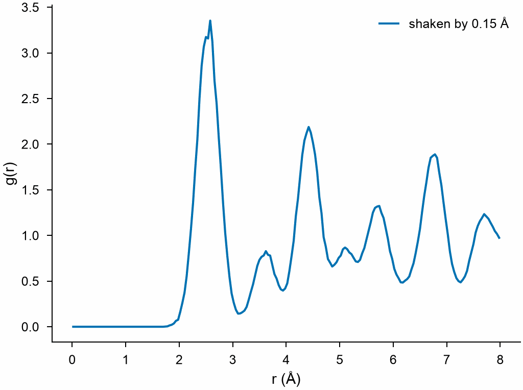
Peaks at the distances between sites of fcc, broadened by the displacements.

The ready-made plots

Common results have a plot of their own, with the labels set. A figure can have several panels:

from mdapy.identify import CommonNeighborAnalysis

structures = CommonNeighborAnalysis().compute(shaken)

with plot.style():
    fig, (left, right) = plot.figure("double", nrows=1, ncols=2)
    plot.rdf(hot, ax=left)
    plot.structure_counts(structures, ax=right)
    plot.panel_label(left, "a")
    plot.panel_label(right, "b")
    plot.save(fig, "images/panels", formats=("png",))

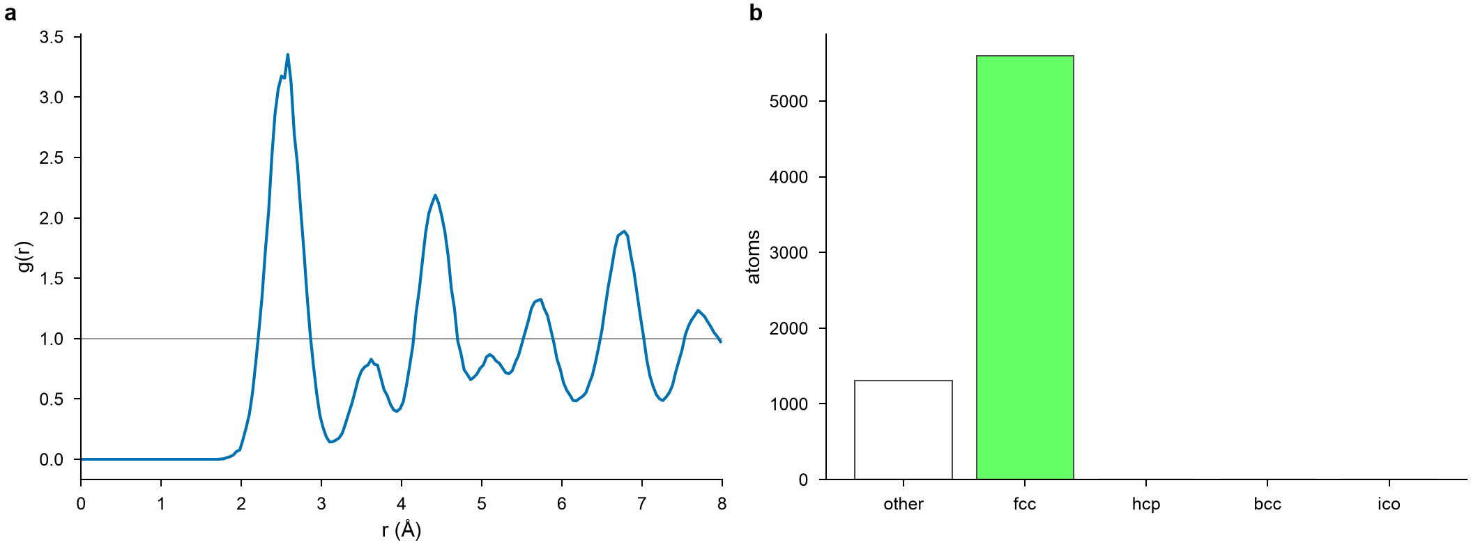
a: g(r) of the shaken crystal. b: its atoms by structure.

Values of the atoms

Histogram gives the distribution of a column. Here, the distance of each atom from its site, computed with the arrays of the two systems:

from mdapy.analysis import Histogram

moved = shaken.with_columns(
    moved=np.linalg.norm(shaken["positions"] - crystal["positions"], axis=1)
)
histogram = Histogram("moved", bins=40).compute(moved)

with plot.style():
    fig, ax = plot.figure("single")
    ax.plot(histogram.center, histogram.counts)
    ax.set_xlabel("Distance moved (Å)")
    ax.set_ylabel("Atoms")
    plot.save(fig, "images/moved", formats=("png",))

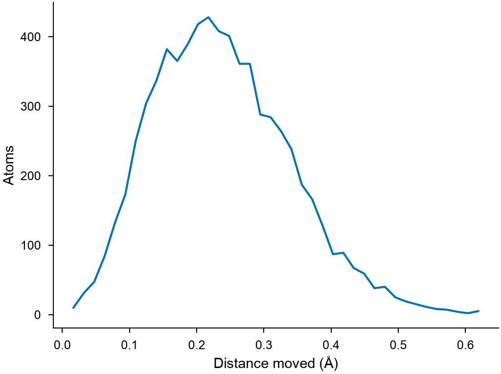
The distribution of the length of a three-dimensional Gaussian step.

Try it

1. Shake the crystal by 0.3 Å and draw both curves in one figure. What happens to the height of the first peak?
2. Save the curve to a text file with np.savetxt("rdf.txt", np.c_[hot.r, hot.g]).

An answer

harder = crystal.with_columns(
    positions=crystal["positions"] + rng.normal(0, 0.3, (len(crystal), 3))
)
hotter = analysis.compute(harder)
with plot.style():
    fig, ax = plot.figure("single")
    ax.plot(hot.r, hot.g, label="0.15 Å")
    ax.plot(hotter.r, hotter.g, label="0.3 Å")
    ax.legend()
    plot.save(fig, "images/two", formats=("png",))

The peak drops to about half and widens by about twice: its area, the number of neighbors, stays.

Next: energies and relaxation. See also Plots, Radial distribution function and Histograms.