Plots¶

mdapy.visualization.plot sets matplotlib up for the figures of journals and plots the results of MDAPY: parity plots of energies and forces, radial distribution functions, structure factors, bond angles, mean squared displacements, stacking fault energies, counts of structures, phonon band structures and densities of states, and two columns of the atoms against each other. It needs matplotlib.

import numpy as np
from mdapy.analysis import RadialDistributionFunction
from mdapy.build import build_crystal, random_alloy
from mdapy.visualization import plot

alloy = random_alloy(
    build_crystal("fcc", 3.6, repeat=(5, 5, 5)), {"Cu": 1, "Ni": 1}, seed=1
)
rdf = RadialDistributionFunction(r_max=8.0, bins=160).compute(alloy)

with plot.style():
    fig, (left, right) = plot.figure("double", nrows=1, ncols=2)
    plot.rdf(rdf, ax=left, partial=True)
    reference = np.random.default_rng(0).normal(size=500)
    plot.parity(
        reference, reference + 0.02, ax=right, label="test", unit="meV/atom", scale=1000
    )
    plot.panel_label(left, "a")
    plot.panel_label(right, "b")
    # plot.save(fig, "figure")  # figure.pdf, figure.svg and figure.png
    fig.savefig("images/plots.png", dpi=200)

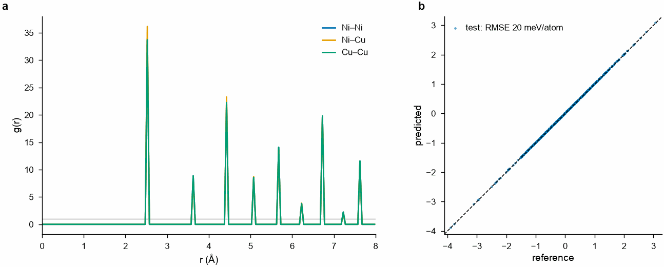
The partial radial distribution functions of a CuNi alloy and a parity plot

a: the partial radial distribution functions of a random CuNi alloy. b: a parity plot with its error in the legend.

In a notebook the figures of a with plot.style(): show when it ends, as the style holds only inside it. Add to a figure, and save it, inside the with.

Columns of the atoms¶

scatter draws two columns of the atoms, components or expressions against each other, a point for each atom: here the number of neighbors of the atoms of a copper nanoparticle, shaken as by heat, against their distance from its center.

from mdapy.analysis import CoordinationNumber

crystal = build_crystal("fcc", 3.615, elements="Cu", repeat=(8, 8, 8))
center = crystal.box.matrix.sum(axis=0) / 2
particle = crystal.filter(np.linalg.norm(crystal["positions"] - center, axis=1) < 12)
rng = np.random.default_rng(1)
particle = particle.with_columns(
    positions=particle["positions"] + rng.normal(0, 0.1, (len(particle), 3))
)
particle = particle.with_columns(
    **CoordinationNumber(cutoff=3.0).compute(particle).columns(),
    distance=np.linalg.norm(particle["positions"] - center, axis=1),
)
with plot.style():
    fig, ax = plot.figure()
    plot.scatter(particle, "distance", "coordination", ax=ax)
    ax.set_xlabel("distance from the center (Å)")
    fig.savefig("images/scatter.png", dpi=200)

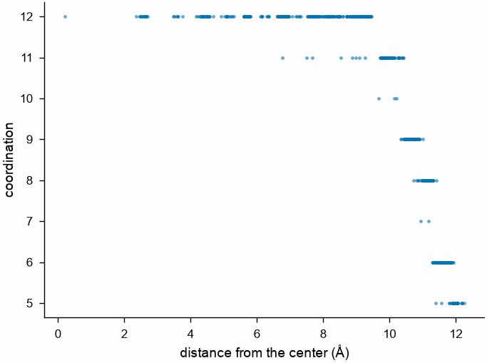
The coordination of the atoms of a nanoparticle against their distance from its center

12 neighbors inside the nanoparticle, fewer at its surface, about 12 Å from its center.

Parameters¶

Function	Does
`style()`	a context in which matplotlib uses `STYLE` and the colors `COLORS`
`figure(width="single", height=None, , nrows=1, ncols=1, *options)`	a figure one column (88 mm) or two (180 mm) wide, or `width` mm; `height` in mm, by default 3/4 of a panel's width per row; `options` go to `plt.subplots`
`panel_label(ax, text, *, x=-0.12, y=1.02)`	a bold label at the top left of a panel
`save(fig, path, formats=("pdf", "svg", "png"))`	the figure in each format, the text of SVG kept as text
`parity(reference, predicted, *, ax=None, label="", unit="", scale=1.0, density=False, color=None)`	predicted against reference values with the diagonal, the root mean square error, times `scale`, in the legend; `density` draws a hexagonal map
`scatter(system, x, y, *, ax=None, atoms=None, max_points=20000, color=None)`	two columns, components or expressions of the atoms (or of those of the mask or indices `atoms`) against each other, as `system[x]` takes them, the atoms with finite values; at most `max_points` of them, picked at random with a fixed seed
`rdf(result, *, ax=None, partial=False)`	g(r), or the partial functions
`structure_factor(result, *, ax=None)`	S(q)
`bond_angles(result, *, ax=None)`	the density of bond angles
`msd(result, *, timestep=1.0, ax=None, fit=None)`	the MSD against time in ps; `fit=(first, last)` fits a line over those lags, its slope over 6 the diffusion coefficient in the legend
`stacking_fault(result, , ax=None, *options)`	a generalized stacking fault energy in mJ/m², a point for each slip joined by a line; `options` go to `ax.plot`, such as `label`
`structure_counts(result, *, ax=None)`	the atoms of each structure type, in its color
`band_structure(result, *, ax=None, color=None)`	phonon frequencies along a path, the special points marked; a color for each branch, or one for all
`phonon_dos(result, *, ax=None, projected=False)`	a phonon density of states, frequencies upward to stand beside a band structure, and that of each atom of the cell

Each plot draws on ax, by default a new figure, and returns the axes.

Results¶

STYLE follows the artwork guides of Nature: sans-serif text of 5 to 7 points, lines of 0.5 to 1 point, no top and right spines, fonts embedded as TrueType. COLORS are those of Okabe and Ito, safe for color blindness. MM, SINGLE and DOUBLE give millimetres and the widths of the columns in inches.

Errors¶

figure raises InvalidParameter for a width that is neither single, double nor a positive number, parity for values of different sizes, and scatter for a column of several components or max_points below 1. Without matplotlib the plots raise ImportError.